Motor Imagery

This tutorial was made by Rakesh C Jakati.

Motor imagery (MI)–based brain-computer interface (BCI) is one of the standard concepts of BCI, in that the user can generate induced activity from the motor cortex by imagining motor movements without any limb movement or external stimulus. In this tutorial, we will learn how to use OpenBCI equipment for motor imagery. For that, we will design a BCI system that allows a user to control a system by imagining different movements of their limbs.

Materials Required

1. OpenBCI Cyton Board
2. Ultracortex EEG headset or EEG cap
3. NodeMCU
4. NodeMCU constructed car
5. Computer with installed with NeuroPype
6. Computer with installed [OpenBCI GUI] (https:)
7. Computer with installed Arduino IDE

Hardware Setup

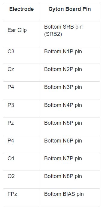
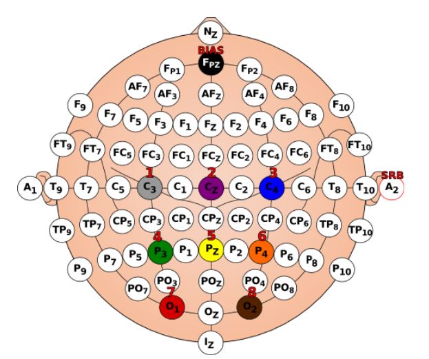
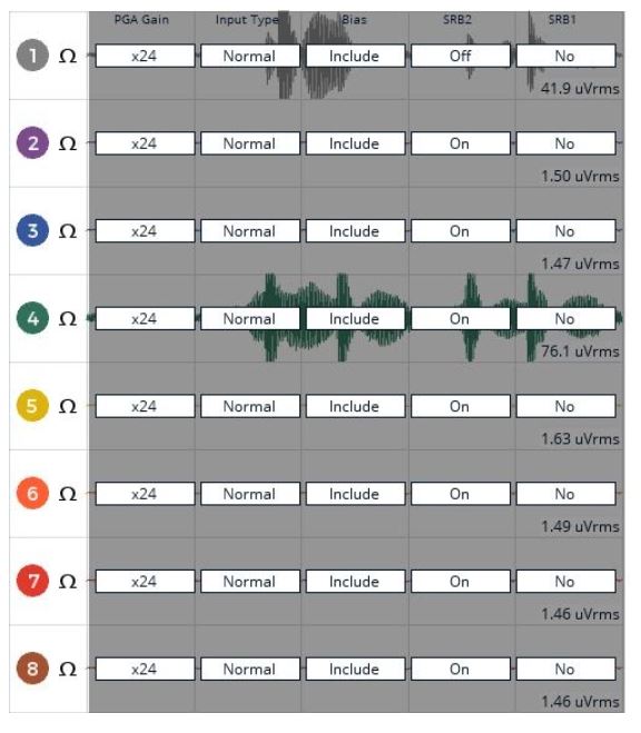
If you are using the assembled Ultracortex IV, all you need to do is place the spiky electrodes on the following 10-20 locations: C3 ,Cz, C4, P3, Pz, P4, O1, O2 and FPz. If you want to assemble the headset yourself follow this tutorial. Next, connect the electrodes to the Cyton board pins as shown on the table below.

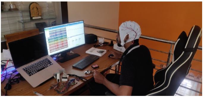
You can either use the EEG Electrode Cap or the Ultracortex Mark IV headset. This demonstration uses a dedicated EEG cap.

Software Setup

Let us design a two-class BCI using the software NeuroPype. NeuroPype is free for academic users and you can get a 30 day trial if you are an individual/startup. You can get started with NeuroPype by clicking here.

When you download Neuropype, several other programs will be installed which we will use in this project.

1. Pipeline Designer
2. Lab Recorder

Python Installation

Download the latest version of miniconda from here.

Open miniconda and create and new environment where you would run all your python scripts. Follow these instruction:

1. conda create -n "openbci_motor_imagery"
2. conda activate openbci_motor_imagery

You should have this environment open and change directory to the required python files to run them. This will be required later in the tutorial.

Imagined Moments Classification

To start open the Neuropype Pipeline Designer application. Go to file and open Simple Motor Imagery Prediction with CSP. We will use the example provided by Neuropype software.

Provided example will be located in: C:\Program File\Intheon\NeuroPype Academic Suite\Examples\SimpleMotorImagery.pyp

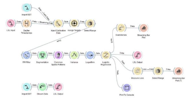
This pipeline uses EEG to predict whether you’re currently imagining one of the possible limb movements (default: left-hand movement vs. right-hand movement for two-class classification). The output of this pipeline at any tick is the probability that the person imagines each type of movement. Since the EEG patterns associated with these movements look different for any two people, several nodes (here: Common Spatial Patterns and Logistic Regression) must first adapt themselves based on some calibration data for the particular user.

Moreover, it’s not enough for the calibration data to be arbitrary EEG data, it must meet certain criteria (this same rule applies to pretty much any use of machine learning on EEG data). First, the node needs to obtain examples of EEG left-hand movement and right-hand movement, respectively. Also, a single trial per class of movement is not enough, the node needs to see close to 20–50 repeats when using a full-sized EEG headset.

Lastly, these trials must be in a randomized order, i.e., not simply a block of all-left trials followed by a block of all-right trials. Collecting data in that way is one of the most common beginner mistakes with machine learning on time series, and it is important to avoid it.

Common Spatial Pattern

Node: Common Spatial Pattern

Change it to 2.

Working with EEG Markers

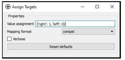
Node: Assign Targets

For the aforementioned reasons, the EEG signal must be annotated such that one can tell which data points correspond to Class 1 (subject imagines left-hand movement) and which ones correspond to Class 2 (subject imagines right-hand movement). One way to do this is to include a special ‘trigger channel’ in the EEG, which takes on pre-defined signal levels that encode different classes (e.g. 0=left, 1=right).

In that case, the pipeline assumes that the data packets emitted by the LSL Input node are not just one EEG stream, but also a second stream that has a list of marker strings along with their timestamps (markers), i.e., they are multi-stream packets and there are consequently two data streams flowing through the entire pipeline.

The markers are then interpreted by the rest of the pipeline to indicate the points in time around which the EEG is of a particular class (in this pipeline, a marker with the string ‘left’ and time-stamp 17.5 would indicate that the EEG at 17.5 seconds into the recording is of class 0, and if the marker had been ‘right’ it would indicate class 1).

Of course, the data could contain any amount of other random markers (e.g., ‘recording-started’, ‘user-was-sneezing’, ‘enter-pressed’), so how does the pipeline know what markers encode classes, and which classes they encode? This binding is established by the Assign Targets node. The settings are shown below. The syntax means that ‘left’ strings map to class 0, ‘right’ maps to class 1, and all other strings don’t map to anything.

Segmentation

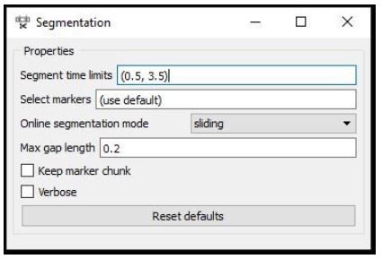
Node: Segmentation

The second question is, given that there’s a marker at 17.5 seconds, how does the pipeline know where relative to that point in time we find the relevant pattern in the EEG that captures the imagined movement? Does it start a second before the marker and end a second after, or does it start at the marker and end 10 seconds later? Extracting the right portion of the data is usually handled by the Segmentation node, which extracts segments of a certain length relative to each marker.

The picture above shows the settings for this pipeline, which are interpreted as follows: extract a segment that starts at 0.5 seconds after each marker and ends at 3.5 seconds after that marker (i.e., the segment is 3 seconds long). If you use negative numbers, you can place the segment before the marker.

Acquition of EEG Data and Markers

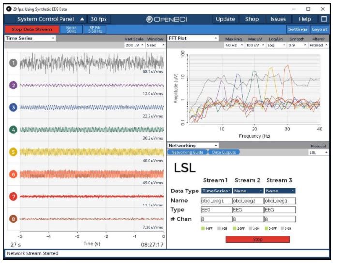
Plug in the RFduino dongle, connect electrodes to the cyton board pins. Wear the EEG headset and finally connect the ear clip to SRB. Open the OpenBCI GUI, select the appropriate port number and start streaming data from the Cyton board. Go to the networking tab and select the LSL protocol. Select “TIME-SERIES” data type and start streaming.

Before we start classifying the Motor Imagery data, we need to calibrate the system.

Recording Calibration Data

Node: Inject Calibration

The NeuroPype pipeline is doing a great job, but wouldn’t it be nice if we didn’t have to recollect the calibration data each time we run the pipeline? It’s often more convenient to record calibration data into a file in the first session, and load that file every time we run our pipeline. For this, we need to use the Inject Calibration Data node, which has a second input port where one can pipe a calibration recording (which we import here using Import XDF).

Start the Lab recorder and find the OpenBCI EEG stream in the window. Now run the python script motorimg_calibrate.py found in the extras folder in your Neuropype installation folder. Now update the streams in the lab recorder. You should now see MotorImag-Markers and obci_eeg1 stream along with your computer name.

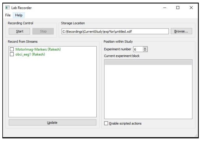
The python script along with OpenBCI, lab recorder is used to record calibration data. The script sends markers matching what the person is imagining that is 'Left' or 'Right' and instructs the user when to imagine that movement which will be stored in the .xdf file along with the EEG data. Run the python script and start recording the OpenBCI stream and markers stream using the lab recorder.

Follow the instructions shown on the window: when the window shows ‘R’  imagine moving your right arm, and when it shows ‘L’   imagine moving your left arm.  It takes about half a second for a person to read the instruction and begin imagining the movement, and he/she will finish about 3 seconds later and get ready for the next trial. This is why the segment time limits in the segmentation node are set to (0.5,3.5). You can configure the number of trials per class and other parameters in motorimg_calibrate.py.

Import Calibration Data

You need to edit a few nodes in this pipeline. You should delete these three nodes (Import SET, Stream Data, LSL Output) at the bottom of the pipeline design as we will use our own recorded calibration data.

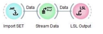Delete these nodes from the Pipeline Design

Delete the Import Set node that is connected to Inject Calibration Data and replace it with Import XDF as the calibration data is recorded in .xdf format. To delete a node select it and press 'delete' key. To add a new node, right click and type 'import xdf'. You can connect a new node to next node by dragging the outer semicircle to the next node.

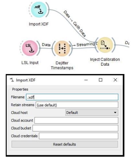
Replace the Import Set with Import XDF

Enter the calibration data filename and fill in the appropriate filename of the XDF file in the window.

Picking up Marker Streams with LSL

Node: LSL Input

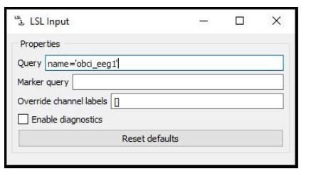
The LSL Input node is responsible for returning a marker stream together with the EEG. Enter the name of the OpenBCI stream in the query and after you import the .xdf calibration data, you are ready to go.

Streaming the Data

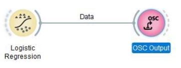
Connect an OSC (Open sound control) Output node to the Logistic Regression node in the pipeline designer and configure it as shown below before you stream the data.

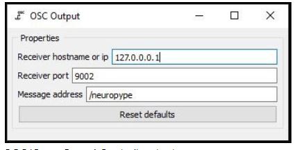
OSC(Open Sound Control) output Type in the IP address of the device to which you want to stream the data, which can be either an Arduino or a Raspberry Pi). Use 127.0.0.1 as an IP address if you want to receive the data on your local computer.

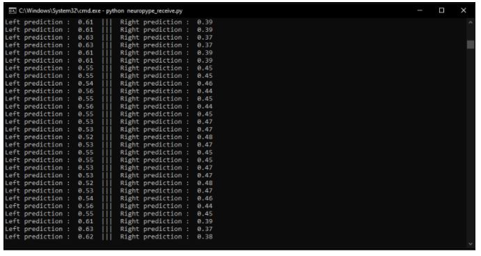
Here is a python code to receive the streamed data on the local computer.

Running NeuroPype Pipeline

We are in the final stage of the Motor Imagery Classification pipeline design. Now right click on the NeuroPype icon in the taskbar and click run pipeline. Navigate to your file path and select your edited pipeline simplemotorimagery.pyp and run it.

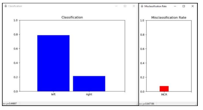
If everything is configured properly, you will get two windows showing the Classification and Misclassification Rate. You can now see real-time predictions of either left or right on the windows. Imagine moving your right arm to increase the amplitude power of the right prediction and imagine moving your left arm to increase the amplitude power of the left prediction.

When you run the python script on your local computer, you should receive the prediction data as shown below.

The car above uses NodeMCU and L298N motor driver. The NodeMCU coded in Arduino IDE and the code is mentioned below. To learn how to use NodeMCU click here.

This OSC protocol is widely used in fields like musical expression, robotics, video performance interfaces, distributed music systems, and inter-process communication. You can use it to drive motors, activate devices, and much more. This example video uses the OSC output to control the direction of rotation of the car.

Following this tutorial, you will be able to design your own Motor Imagery Classification with your own calibration data and control cars, drones, and devices. Start using BCI technologies to bring products of your imagination to life - there is no limit to what you can imagine!